![]()
The days where marketers made changes to their websites based on gut-feelings alone are far behind us. We are now deep in the A/B testing era, basing our decisions on as much empirical data as possible.
To enable that, the community has looked for A/B testing tools to help us make informed decisions based on collected data. Or, in more exact terms: to soundly generalize from observed data and gain insight into the future.
The aim of this post is to discuss the evolution these tools are currently undergoing, from the basic “frequentist” testing method used in the past (and still commonly used today) to the new Bayesian testing method which the industry is moving toward.
Underlying these two approaches is a different viewpoint on what probability is. I will attempt to highlight that difference and the practical implications it has, but without delving into the hard-core math.
At the dawn of the A/B testing era, statisticians provided a very basic framework for statistical inference in an A/B testing scenario. Commonly known as “Hypothesis Testing,” the procedure goes as follows:
People tend to think that the p-value represents the probability that variation B is really better than A. However, this is a common misinterpretation; It actually has to do with the hypothesis that is at the base of Hypothesis Testing.
What p-value tests for is not the “optimistic” case in which our alternative variation B is really better than the baseline. Instead, we start with a pessimistic hypothesis (called the “Null Hypothesis”) stating that the newly introduced variation B is not any better than the existing baseline A, and that the observed differences represent no more than random noise.
We then try to reject this hypothesis by calculating how rare our empirical findings are if the above Null Hypothesis is correct. The p-value represents that probability.
If the p-value is below a certain threshold (often taken as 0.05), we can state that our finding allows us to reject the Null Hypothesis and thus declare variation B as the winner. In addition, this Hypothesis Testing framework provides a way to calculate a confidence interval, which is aimed at getting a sense of how confident we are that the measured values will last for the long haul.
Take a moment and notice how convoluted and unintuitive this whole framework is.
It requires a known baseline and reaching a predefined sample size before we’re allowed to look at the data and draw conclusions. These conclusions are based on metrics that, to paraphrase Inigo Montoya in the “Princess Bride,” do not mean what most people think they mean.
This begs the question: can we do something to make things simpler, less restrictive, more reliable and more intuitive? The answer is yes.
In the field of statistical inference, there are two very different, yet mainstream, schools of thought: the frequentist approach, under which the framework of Hypothesis Testing was developed, and the Bayesian approach, which I’d like to introduce to you now.
The difference between these two rival schools can be explained through the different interpretation each gives to the term probability. The intro given here is adapted from this series of blog posts.
Let’s take a concrete case-in-point: say we are interested in discovering the average height of American citizens nowadays. For a frequentist, this number is unknown but fixed. This is a natural intuitive view, as you can imagine that if you go through all American citizens one by one, measure their height and average the list, you will get the actual number.
However, since you do not have access to all American citizens, you take a sample of, say, a thousand citizens, measure and average their height to produce a point estimate, and then calculate the estimate of your error. The point is that the frequentist looks at the average height as a single unknown number.
A Bayesian statistician, however, would have an entirely different take on the situation. A Bayesian would look at the average height of an American citizen not as a fixed number, but instead as an unknown distribution (you might imagine here a “bell” shaped normal distribution).
Initially, the Bayesian statistician has some basic prior knowledge which is being assumed: for example, that the average height is somewhere between 50cm and 250cm.
Then, the Bayesian begins to measure heights of specific American citizens, and with each measurement updates the distribution to become a bit more “bell-shaped” around the average height measured so far. As more data is collected, the “bell” becomes sharper and more concentrated around the measured average height.
For Bayesians, probabilities are fundamentally related to their knowledge about an event. This means, for example, that in a Bayesian view, we can meaningfully talk about the probability that the true conversion rate lies in a given range, and that probability codifies our knowledge of the value based on prior information and/or available data.
For Bayesians, the concept of probability is extended to cover degrees of certainty about any given statement on reality. However, in a strict frequentist view, it is meaningless to talk about the probability of the true conversion rate. For frequentists, the true conversion rate is by definition a single fixed number, and to talk about a probability distribution for a fixed number is mathematically nonsensical.
The same logic applies when seeking to measure the conversion rate of a web-based purchase funnel. Sure, probability can certainly be estimated in a frequentist fashion by measuring the ratio of how many times a conversion was made out of a huge number of trials. But this is not fundamental to the Bayesian, who can stop the test at any point and calculate probabilities from data.
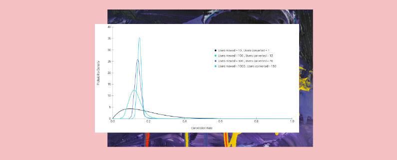
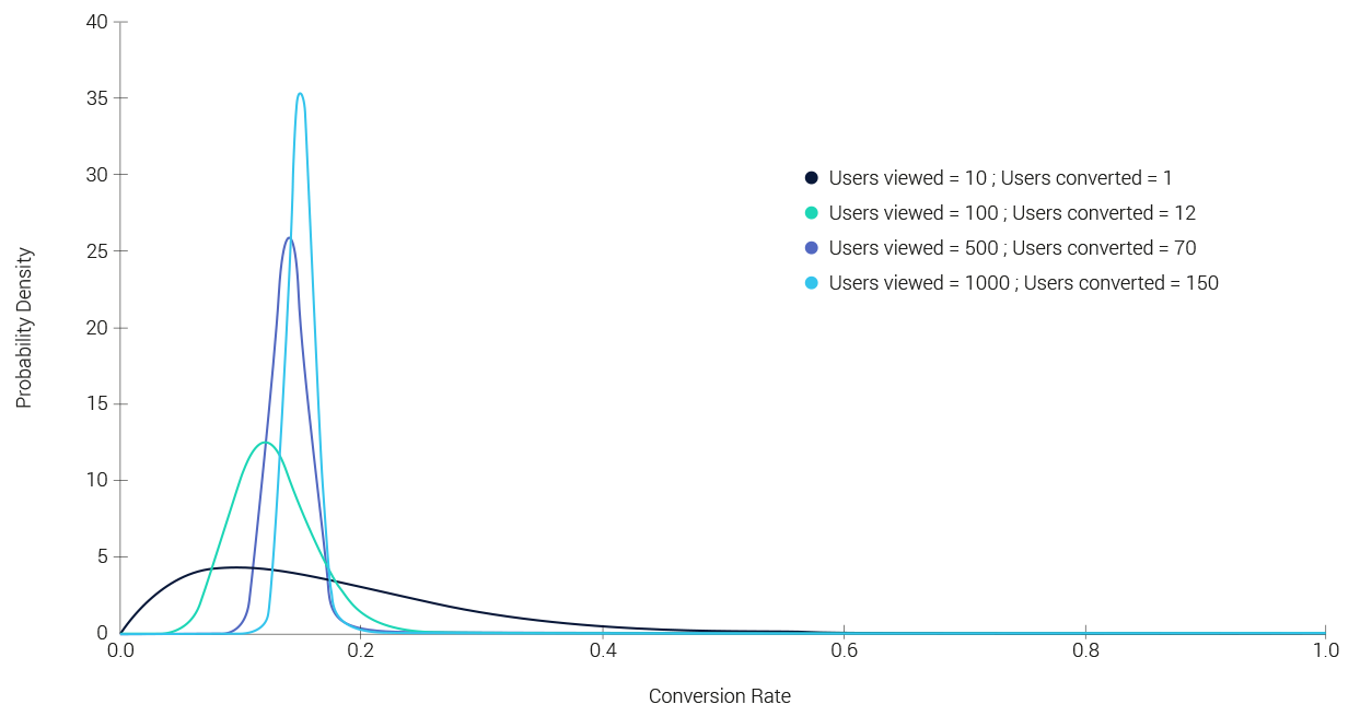
To illustrate the convergence process of the distribution as more data is collected, here is a plot based on test data. Notice how the bell shape becomes sharper (more certain) as data streams in:
The surprising thing is that this arguably subtle difference in philosophy between these schools leads in practice to vastly different approaches to the statistical analysis of data.
The math behind the Bayesian framework is quite complex so I will not get into it here. In fact, I would argue that the fact that the math is more complicated than can be computed with a simple calculator or Microsoft Excel is a dominant factor in the slow adoption of this method in the industry.
The framework involves some daunting terms such as Prior, Posterior, Bayes Theorem, Beta and Gamma distributions, Monte Carlo Integration, and more.
However, if we look at the Bayesian statistical engine as a “mathematical black box”, we will see that the inputs to it, and more importantly the outputs from it, are actually quite simple and intuitive. An input/output diagram of the engine would look something like this:
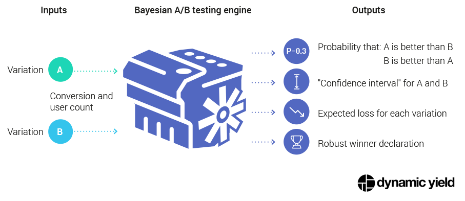
Although we’re not delving into specifics, you can immediately see that the Bayesian engine provides answers to more direct questions such as:
What is the probability that A is better than B? (contrast this with the contrived p-value mentioned earlier)
If I declare B as a winner, and it is not really better, how much should I expect to lose in terms of conversion rate?
Also, this engine can emit a new kind of “confidence interval” metric, mathematically termed Highest Posterior Density Region (HPDR). This provides an answer to a pretty intuitive requirement, namely: give me the conversion rate boundaries (interval) in which the true conversion rate falls with (say) 95% probability.
If we want to be exact about the meaning of the oft-used frequentist confidence interval, it means roughly the following: “if we would have repeated this test many times, and would have calculated a different confidence interval for each case, then in 95% of the times the actual conversion rate would fall within this interval.” How is that for intuitiveness? 🙂
Let’s summarize how the two frameworks compare:
| Hypothesis Testing | Bayesian A/B Testing | |
| Knowledge of Baseline Performance | Required | Not Required |
| Intuitiveness | Less, as p-value is a convoluted term | More, as we directly calculate the probability of A being better than B |
| Sample size | Pre-defined | No need to pre-define |
| Peeking at the data while the test runs | Not allowed | Allowed (with caution) |
| Quick to make decisions | Less, as it has more restrictive assumptions on distributions | More, as it has less restrictive assumptions |
| Representing uncertainty | Confidence Interval (again, a convoluted interpretation which is often misunderstood) | Highest Posterior Density Region – highly intuitive interpretation |
| Declaring a winner | When sample size is reached and p-value is below a certain threshold | When either “probability to be best” goes above a threshold or the expected loss is below a threshold (in which case a “tie” can be declared between multiple variations) |
I should note, though, that generally speaking, a frequentist A/B testing framework which performs as well as the Bayesian framework described here is possible, but further development would be needed above what is usually implemented.
To conclude, the industry is moving toward the Bayesian framework as it is a simpler, less restrictive, more reliable and more intuitive approach to A/B testing.
P.S. Here at Dynamic Yield, we have made the move to a Bayesian statistical engine not only for binary objectives such as goal conversion rate and CTR but also for non-binary objectives such as Revenue Per User (which merits a future blog post in its own right). With this new engine, our customers now benefit from a quicker and more robust statistical engine.
